OZONE LAYER

Ozone layer

The ozone layer is a layer in Earth's atmosphere which contains relatively high concentrations of ozone (O₃). This layer absorbs 97–99% of the Sun's high frequency ultraviolet light, which is potentially damaging to life on Earth. It is mainly located in the lower portion of the stratosphere from approximately 13 km to 40 km above Earth, though the thickness varies seasonally and geographically. The ozone layer was discovered in 1913 by the French physicistsCharles Fabry and Henri Buisson. Its properties were explored in detail by the British meteorologist G. M. B. Dobson, who developed a simple spectrophotometer (the Dobsonmeter) that could be used to measure stratospheric ozone from the ground. Between 1928 and 1958 Dobson established a worldwide network of ozone monitoring stations which continues to operate today. The "Dobson unit", a convenient measure of the columnar density of ozone overhead, is named in his honor.

Origin of ozone

Ozone-oxygen cycle in the ozone layer.

The photochemical mechanisms that give rise to the ozone layer were discovered by the British physicist Sidney Chapman in 1930. Ozone in the Earth's stratosphere is created by ultraviolet light striking oxygen molecules containing two oxygen atoms (O₂), splitting them into individual oxygen atoms (atomic oxygen); the atomic oxygen then combines with unbroken O₂ to create ozone, O₃. The ozone molecule is also unstable (although, in the stratosphere, long-lived) and when ultraviolet light hits ozone it splits into a molecule of O₂ and an atom of atomic oxygen, a continuing process called the ozone-oxygen cycle, thus creating an ozone layer in the stratosphere, the region from about 10 to 50 km (32,000 to 164,000 feet) above Earth's surface. About 90% of the ozone in our atmosphere is contained in the stratosphere. Ozone concentrations are greatest between about 20 and 40 km, where they range from about 2 to 8 parts per million. If all of the ozone were compressed to the pressure of the air at sea level, it would be only a few millimeters thick

Ultraviolet light and ozone

Levels of ozone at various altitudes and blocking of ultraviolet radiation.

UV-B energy levels at several altitudes. Blue line shows DNA sensitivity. Red line shows surface energy level with 10% decrease in ozone

Although the concentration of the ozone in the ozone layer is very small, it is vitally important to life because it absorbs biologically harmful ultraviolet (UV) radiation coming from the Sun. UV radiation is divided into three categories, based on its wavelength; these are referred to as UV-A (400–315 nm), UV-B (315–280 nm), and UV-C (280–100 nm). UV-C, which would be very harmful to all living things, is entirely screened out by ozone at around 35 km altitude. UV-B radiation can be harmful to the skin and is the main cause of sunburn; excessive exposure can also cause genetic damage, resulting in problems such as skin cancer. The ozone layer is very effective at screening out UV-B; for radiation with a wavelength of 290 nm, the intensity at the top of the atmosphere is 350 million times stronger than at the Earth's surface. Nevertheless, some UV-B reaches the surface. Most UV-A reaches the surface; this radiation is significantly less harmful, although it can potentially cause genetic damage.

Distribution of ozone in the stratosphere

The thickness of the ozone layer—that is, the total amount of ozone in a column overhead—varies by a large factor worldwide, being in general smaller near the equator and larger towards the poles. It also varies with season, being in general thicker during the spring and thinner during the autumn in the northern hemisphere. The reasons for this latitude and seasonal dependence are complicated, involving atmospheric circulation patterns as well as solar intensity.

Since stratospheric ozone is produced by solar UV radiation, one might expect to find the highest ozone levels over the tropics and the lowest over Polar Regions. The same argument would lead one to expect the highest ozone levels in the summer and the lowest in the winter. The observed behavior is very different: most of the ozone is found in the mid-to-high latitudes of the northern and southern hemispheres, and the highest levels are found in the spring, not summer, and the lowest in the autumn, not winter in the northern hemisphere. During winter, the ozone layer actually increases in depth. This puzzle is explained by the prevailing stratospheric wind patterns, known as the Brewer-Dobson circulation. While most of the ozone is indeed created over the tropics, the stratospheric circulation then transports it pole ward and downward to the lower stratosphere of the high latitudes. However in the southern hemisphere, owing to the ozone hole phenomenon, the lowest amounts of column ozone found anywhere in the world are over the Antarctic in the southern spring period of September and October.

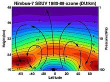
Brewer-Dobson circulation in the ozone layer.

The ozone layer is higher in altitude in the tropics, and lower in altitude in the extra tropics, especially in the Polar Regions. This altitude variation of ozone results from the slow circulation that lifts the ozone-poor air out of the troposphere into the stratosphere. As this air slowly rises in the tropics, ozone is produced by the overhead sun which photolyzes oxygen molecules. As this slow circulation bends towards the mid-latitudes, it carries the ozone-rich air from the tropical middle stratosphere to the mid-and-high latitudes lower stratosphere. The high ozone concentrations at high latitudes are due to the accumulation of ozone at lower altitudes.

The Brewer-Dobson circulation moves very slowly. The time needed to lift an air parcel from the tropical tropopause near 16 km (50,000 ft) to 20 km is about 4–5 months (about 30 feet (9.1 m) per day). Even though ozone in the lower tropical stratosphere is produced at a very slow rate, the lifting circulation is so slow that ozone can build up to relatively high levels by the time it reaches 26 km.

Ozone amounts over the continental United States (25°N to 49°N) are highest in the northern spring (April and May). These ozone amounts fall over the course of the summer to their lowest amounts in October, and then rise again over the course of the winter. Again, wind transport of ozone is principally responsible for the seasonal evolution of these higher latitude ozone patterns.

The total column amount of ozone generally increases as we move from the tropics to higher latitudes in both hemispheres. However, the overall column amounts are greater in the northern hemisphere high latitudes than in the southern hemisphere high latitudes. In addition, while the highest amounts of column ozone over the Arctic occur in the northern spring (March–April), the opposite is true over the Antarctic, where the lowest amounts of column ozone occur in the southern spring (September–October).

Ozone depletion

NASA projections of stratospheric ozone concentrations if chlorofluorocarbons had not been banned.

The ozone layer can be depleted by free radical catalysts, including nitric oxide (NO), nitrous oxide (N₂O), hydroxyl(OH), atomic chlorine (Cl), and atomic bromine (Br). While there are natural sources for all of these species, the concentrations of chlorine and bromine have increased markedly in recent years due to the release of large quantities of man-made organohalogen compounds, especially chlorofluorocarbons (CFCs) and bromofluorocarbons. These highly stable compounds are capable of surviving the rise to the stratosphere, where Cl and Br radicals are liberated by the action of ultraviolet light. Each radical is then free to initiate and catalyze a chain reaction capable of breaking down over 100,000 ozone molecules. The breakdown of ozone in the stratosphere results in the ozone molecules being unable to absorb ultraviolet radiation. Consequently, unabsorbed and dangerous ultraviolet-B radiation is able to reach the Earth’s surface. Ozone levels, over the northern hemisphere, have been dropping by 4% per decade. Over approximately 5% of the Earth's surface, around the north and south poles, much larger (but seasonal) declines have been seen; these are the ozone holes.

In 2009, nitrous oxide (N₂O) was the largest ozone-depleting substance emitted through human activities.

Regulation

In 1978, the United States, Canada and Norway enacted bans on CFC-containing aerosol sprays that are thought to damage the ozone layer. The European Community rejected an analogous proposal to do the same. In the U.S., chlorofluorocarbons continued to be used in other applications, such as refrigeration and industrial cleaning, until after the discovery of the Antarctic ozone hole in 1985. After negotiation of an international treaty (the Montreal Protocol), CFC production was sharply limited beginning in 1987 and phased out completely by 1996^.

On August 2, 2003, scientists announced that the depletion of the ozone layer may be slowing down due to the international ban on CFCs. Three satellites and three ground stations confirmed that the upper atmosphere ozone depletion rate has slowed down significantly during the past decade. The study was organized by the American Geophysical Union. Some breakdown can be expected to continue due to CFCs used by nations which have not banned them, and due to gases which are already in the stratosphere. CFCs have very long atmospheric lifetimes, ranging from 50 to over 100 years, so the final recovery of the ozone layer is expected to require several lifetimes.

Compounds containing C–H bonds have been designed to replace the function of CFC's (such as HCFC), since these compounds are more reactive and less likely to survive long enough in the atmosphere to reach the stratosphere where they could affect the ozone layer. While being less damaging than CFC's, HCFC's also have a significant negative impact on the ozone layer. HCFC's are also being phased out.

SOLAR WIND

The solar wind is a stream of charged particles ejected from the upper atmosphere of the Sun. It mostly consists of electrons and protons with energies usually between 10 and 100 keV. The stream of particles varies in temperature and speed over time. These particles can escape the Sun’s gravity because of their high kinetic energy and the high temperature of the corona.

The solar wind creates the heliosphere, a vast bubble in the interstellar medium that surrounds the solar system. Other phenomena include geomagnetic that can knock out power grids on Earth, the aurorae (northern and southern lights), and the plasma tails of comets that always point away from the Sun.

HISTORY

The continuous stream of particles flowing outward from the Sun was first suggested by British astronomer Richard C. Carrington. In 1859, Carrington and Richard Hodgson independently made the first observation of what would later be called a solar flare. This is a sudden outburst of energy from the Sun's atmosphere. On the following day, a geomagnetic storm was observed, and Carrington suspected that there may be a connection. George Fitzgerald later suggested that matter was being regularly accelerated away from the Sun and was reaching the Earth after several days.

Laboratory simulation of the magnetosphere's influence on the Solar Wind; these auroral-likeBirkeland currents were created in a terrella, a magnetised anode globe in an evacuated chamber.

The ideas of Fitzgerald and others were further developed by the Norwegian physicist Kristian Birkeland. His geomagnetic surveys showed that auroral activity was nearly uninterrupted. As these displays and other geomagnetic activity were being produced by particles from the Sun, he concluded that the Earth was being continually bombarded by "rays of electric corpuscles emitted by the Sun". In 1916, Birkeland was probably the first person to successfully predict that, "From a physical point of view it is most probable that solar rays are neither exclusively negative nor positive rays, but of both kinds". In other words, the solar wind consists of both negative electrons and positive ions. Three years later in 1919, Frederick Lindemann also suggested that particles of polarities, protons as well as electrons, come from the Sun.

Around the 1930s, scientists had determined that the temperature of the solar corona must be a million degrees Celsius because of the way it stood out into space (as seen during total eclipses). Later spectroscopic work confirmed this extraordinary temperature. In the mid-1950s the British mathematician Sydney Chapman calculated the properties of a gas at such a temperature and determined it was such a superb conductor of heat that it must extend way out into space, beyond the orbit of Earth. Also in the 1950s, a German scientist named Ludwig Biermann became interested in the fact that no matter whether a comet is headed towards or away from the Sun, its tail always points away from the Sun. Biermann postulated that this happens because the Sun emits a steady stream of particles that pushes the comet's tail away. Wilfried Schröder claims in his book, Who First Discovered the Solar Wind?, that the German astronomer Paul Ahnert was the first to relate solar wind to comet tail direction based on observations of the comet Whipple-Fedke (1942g).

Eugene Parker realized that the heat flowing from the Sun in Chapman's model and the comet tail blowing away from the Sun in Biermann's hypothesis had to be the result of the same phenomenon, which he termed the "solar wind". Parker showed that even though the Sun's corona is strongly attracted by solar gravity, it is such a good conductor of heat that it is still very hot at large distances. Since gravity weakens as distance from the Sun increases, the outer coronal atmosphere escapes supersonically into interstellar space. Furthermore, Parker was the first person to notice that the weakening effect of the gravity has the same effect on hydrodynamic flow as a de Laval nozzle: it incites a transition from subsonic to supersonic flow.

Opposition to Parker's hypothesis on the solar wind was strong. The paper he submitted to the Astrophysical Journal in 1958 was rejected by two reviewers. It was saved by the editor Subrahmanyan Chandrasekhar (who later received the 1983 Nobel Prize in physics).

In January 1959, the Soviet satellite Luna 1 first directly observed the solar wind and measured its strength. They were detected by hemispherical ion traps. The discovery, made by Konstantin Gringauz, was verified by Luna 2, Luna 3 and by the more distant measurements of Venera 1. Three years later its measurement was performed by Americans (Neugebauer and collaborators) using the Mariner 2spacecraft.

However, the acceleration of the fast wind is still not understood and cannot be fully explained by Parker's theory. The first numerical simulation of the solar wind in the solar corona including closed and open field lines was performed by Pneuman and Knopp in 1971. Themagnetohydrodynamics equations in steady state were solved iteratively starting with an initial dipolar configuration.

In the late 1990s the Ultraviolet Coronal Spectrometer (UVCS) instrument on board the SOHO spacecraft observed the acceleration region of the fast solar wind emanating from the poles of the Sun, and found that the wind accelerates much faster than can be accounted for by thermodynamic expansion alone. Parker's model predicted that the wind should make the transition to supersonic flow at an altitude of about 4 solar radii from the photosphere; but the transition (or "sonic point") now appears to be much lower, perhaps only 1 solar radius above the photosphere

suggesting that some additional mechanism accelerates the solar wind away from the Sun.

In 1990, the Ulysses probe was launched to study the solar wind from high solar latitudes. All prior observations had been made at or near the solar system's ecliptic plane.

EMISSION

While early models of the solar wind used primarily thermal energy to accelerate the material, by the 1960s it was clear that thermal acceleration alone cannot account for the high speed of solar wind. An additional unknown acceleration mechanism is required, and likely relates to magnetic fields in the solar atmosphere.

The Sun's corona, or extended outer layer, is a region of plasma that is heated to over a million degrees Celsius. As a result of thermal collisions, the particles within the inner corona have a range and distribution of speeds described by a Maxwellian distribution. The mean velocity of these particles is about 145 km/s, which is well below the solar escape velocity of 618 km/s. However, a few of the particles achieve energies sufficient to reach the terminal velocity of 400 km/s, which allows them to feed the solar wind. At the same temperature, electrons, due to their much smaller mass, reach escape velocity and build up an electric field that further accelerates ions - charged atoms - away from the Sun.

The total number of particles carried away from the Sun by the solar wind is about 1.3 × 10³⁶ per second. Thus, the total mass loss each year is about (2–3) × 10⁻¹⁴ solar masses, or 6.7 billion tons per hour. This is equivalent to losing a mass equal to the Earth every 150 million years. However, only about 0.01% of the Sun's total mass has been lost through the solar wind. Other stars have much stronger stellar winds that result in significantly higher mass loss rates.

Components

The solar wind is divided into two components, respectively termed the slow solar wind and the fast solar wind. The slow solar wind has a velocity of about 400 km/s, a temperature of 1.4–1.6 × 10⁶ K and a composition that is a close match to the corona. By contrast, the fast solar wind has a typical velocity of 750 km/s, a temperature of 8 × 10⁵ K and it nearly matches the composition of the Sun's photosphere. The slow solar wind is twice as dense and more variable in intensity than the fast solar wind. The slow wind also has a more complex structure, with turbulent regions and large-scale structures.

The slow solar wind appears to originate from a region around the Sun's equatorial belt that is known as the "streamer belt". Coronal streamers extend outward from this region, carrying plasma from the interior along closed magnetic loops. Observations of the Sun between 1996 and 2001 showed that emission of the slow solar wind occurred between latitudes of 30–35° around the equator during the solar (the period of lowest solar activity), then expanded toward the poles as the minimum waned. By the time of the solar maximum, the poles were also emitting a slow solar wind.

The fast solar wind is thought to originate from coronal holes, which are funnel-like regions of open field lines in the Sun's magnetic field. Such open lines are particularly prevalent around the Sun's magnetic poles. The plasma source is small magnetic fields created by convection in the solar atmosphere. These fields confine the plasma and transport it into the narrow necks of the coronal funnels, which are located only 20,000 kilometers above the photosphere. The plasma is released into the funnel when these magnetic field lines reconnect.

Coronal mass ejection

Both the fast and slow solar wind can be interrupted by large, fast-moving bursts of plasma called interplanetary coronal mass ejections, or ICMEs. ICMEs are the interplanetary manifestation of solar coronal mass ejections, which are caused by release of magnetic energy at the Sun. CMEs are often called "solar storms" or "space storms" in the popular media. They are sometimes, but not always, associated with solar flares, which are another manifestation of magnetic energy release at the Sun. ICMEs cause shock waves in the thin plasma of the heliosphere, launching electromagnetic waves and accelerating particles (mostly protons and electrons) to form showers of radiation that precede the CME.

When an CME impacts the Earth's magnetosphere, it temporarily deforms the Earth's magnetic field, changing the direction of compass needles and inducing large electrical ground currents in Earth itself; this is called a geomagnetic storm and it is a global phenomenon. CME impacts can induce magnetic reconnection in Earth's magneto tail (the midnight side of the magnetosphere); this launches protons and electrons downward toward Earth's atmosphere, where they form the aurora.

ICMEs are not the only cause of space weather. Different patches on the Sun are known to give rise to slightly different speeds and densities of wind depending on local conditions. In isolation, each of these different wind streams would form a spiral with a slightly different angle, with fast-moving streams moving out more directly and slow-moving streams wrapping more around the Sun. Faster-moving streams tend to overtake slower streams that originate westward of them on the sun, forming turbulent co-rotating interaction regions that give rise to wave motions and accelerated particles, and that affect Earth's magnetosphere in the same way as, but more gently than, CMEs.

EFFECTS ON THE SOLAR SYSTEM

Over the lifetime of the Sun, the surface rotation rate has decreased significantly. This loss of rotation is thought to have been caused by interaction of the Sun's surface layers with the escaping solar wind. The wind is considered responsible for the tails of comets, along with the Sun's radiation. The solar wind contributes to fluctuations in celestial radio waves observed on the Earth, through an effect called interplanetary scintillation.

Magnetospheres

As the solar wind approaches a planet that has a well-developed magnetic field (such as Earth, Jupiter and Saturn), the particles are deflected by the Lorentz force. This region, known as the magnetosphere, causes the particles to travel around the planet rather than bombarding the atmosphere or surface. The magnetosphere is roughly shaped like a hemisphere on the side facing the Sun, then is drawn out in a long wake on the opposite side. The boundary of this region is called the magnetopause, and some of the particles are able to penetrate the magnetosphere through this region by partial reconnection of the magnetic field lines.

Earth itself is largely protected from the solar wind by its magnetic field, which deflects most of the charged particles, however some of the charged particles are trapped in the Van Allen radiation belt. A smaller number of particles from the solar wind manage to travel, as though on an electromagnetic energy transmission line, to the Earth's upper atmosphere and ionosphere in the auroral zones. The only time the solar wind is observable on the Earth is when it is strong enough to produce phenomena such as the aurora and geomagnetic storms. Bright auroras strongly heat the ionosphere, causing its plasma to expand into the magnetosphere, increasing the size of the plasma geosphere, and causing escape of atmospheric matter into the solar wind. Geomagnetic storms result when the pressure of plasmas contained inside the magnetosphere is sufficiently large to inflate and thereby distort the geomagnetic field.

The solar wind is responsible for the overall shape of Earth's magnetosphere, and fluctuations in its speed, density, direction, and entrained magnetic field strongly affect Earth's local space environment. For example, the levels of ionizing radiation and radio interference can vary by factors of hundreds to thousands; and the shape and location of the magnetopause and bow shock wave upstream of it can change by several Earth radii, exposing geosynchronous satellites to the direct solar wind. These phenomena are collectively called space weather.

Atmospheres

The solar wind affects the other incoming cosmic rays interacting with the atmosphere of planets. Moreover, planets with a weak or non-existent magnetosphere are subject to atmospheric stripping by the solar wind.

Venus, the nearest and most similar planet to Earth in our solar system, has an atmosphere 100 times denser than our own. Modern space probes have discovered a comet-like tail that extends to the orbit of the Earth.

Mars is larger than Mercury and four times farther from the Sun, and yet even here it is thought that the solar wind has stripped away up to a third of its original atmosphere, leaving a layer 1/100th as dense as the Earth's. It is believed the mechanism for this atmospheric stripping is gas being caught in bubbles of magnetic field, which are ripped off by solar winds.

Planetary surfaces

Mercury, the nearest planet to the Sun, bears the full brunt of the solar wind, and its atmosphere is vestigial and transient, its surface bathed in radiation.

The Earth's Moon has no atmosphere or intrinsic magnetic field, and consequently its surface is bombarded with the full solar wind. The Project Apollo missions deployed passive aluminum collectors in an attempt to sample the solar wind, and lunar soil returned for study confirmed that the lunar regolith is enriched in atomic nuclei deposited from the solar wind. There has been speculation that these elements may prove to be useful resources for future lunar colonies.

OUTER LIMITS

The solar wind "blows a bubble" in the interstellar medium (the rarefied hydrogen and helium gas that permeates the galaxy). The point where the solar wind's strength is no longer great enough to push back the interstellar medium is known as the heliopause, and is often considered to be the outer "border" of the solar system. The distance to the heliopause is not precisely known, and probably varies widely depending on the current velocity of the solar wind and the local density of the interstellar medium, but it is known to lie far outside the orbit of Pluto. Scientists hope to gain more perspective on the heliopause from data acquired through the Interstellar Boundary Explorer (IBEX) mission, launched in October 2008.

NOBEL EVENTS

§ From May 10, 1999 to May 12, NASA's ACE and Wind spacecraft observed a 98% decrease of solar wind density. This allowed energetic electrons from the Sun to flow to Earth in narrow beams known as "strahl", which caused a highly unusual "polar rain" event, in which a visible aurora appeared over the North Pole. In addition, Earth's magnetosphere increased to between 5 and 6 times its normal size.

VEHICLES WITHOUT DRIVERS

What Is HAARP?

What Is HAARP?

The official HAARP facility is located in Gakuna, Alaska. The site consists of a collection of antennae, arranged in a computer-controlled grid, known as a "phased array." A phased array has the ability to focus radio signals in a precise direction, without the necessity of turning the antennae. Modern radar systems no longer use the revolving dish that we have come to recognize. The new radar antennae, which rely on phased arrays, look more like the flat screen of a drive-in movie, speckled with small umbrella-like antennae in neat rows. The phased array in HAARP is not a radar, but it uses some of the same extremely high frequencies to focus a powerful radio beam to specific locations in the Earth's ionosphere.

The ionosphere is a layer of charged particles (or "ions") located about 60-90 kilometers above the Earth's surface. It is the layer which reflects short wave radio waves and makes it possible for a transmitter in New York to send a signal to Tokyo. Short waves may be good enough to send The Voice of America broadcasts, but they are subject to noise and static. Short wave signals lose much of their power as they travel and can even be blocked by the weather and sunspot activity.

Extremely High Frequency waves, on the other hand, aremuch shorter than short waves. They travel in compact, narrowly focused, beams. They do not encounter static or deteriorate from rain or clouds. Since they retain their strength over long distances, they are preferred for most point-to-point communications. Unfortunately, though, EHF waves (including microwaves) do not naturally reflect and bounce off of the ionosphere. For this reason, high frequency waves are said to propagate along the "line of sight." If you own a satellite television dish, you know that it is important for your antenna to be pointed in the direction of the satellite. This is because you are receiving extremely high frequency waves.

Eastlund's discovery involved beaming High Frequency (HF) and Extremely High Frequency (EHF) waves, of extremely high power (over a billion watts), directly at a point on the ionosphere. When this was done, the ionosphere became heated from the accumulating electrical energy. You might think of it as "cooking" the atmosphere.

The heated portion of the ionosphere expands like heated plastic and is raised to a higher altitude, causing an atmospheric "bulge." Eastlund discovered that this bulge was highly reflective to radio waves, and, because of its altitude, it could bounce high frequency radio signals to points well beyond the horizon. Even efficient ELF and microwaves signals, which normally would pass through the ionosphere into space, could be deflected without much loss of strength. He called this heated "bulge" the "lens effect."

Eastlund's first patent (US #4,686,605) was for a "method and apparatus for altering a region in the Earth's atmosphere, ionosphere, and or magnetosphere." His second patent described the reflection of a second signal, using the ionospheric bulge, to distant locations on the Earth's surface. Eastlund had been working with the Atlantic Richfield Company, holders of a massive reserve of natural gas under Alaska's north slope. ARCO bought Eastlund's first two patents with the understanding that this new technology would make it possible for their natural gas reserves, too expensive to be piped from Alaska, to be converted to electrical energy on the north slope, and then bounced off the heated ionosphere to customers in remote locations around the globe. Also, because Eastlund's "heaters" could elevate the Earth's ionosphere, his discovery provided the ability to control weather! Jet streams could be altered, tornadoes could be zapped and rain could be made-- anywhere and anytime-- right here and right now! But the military had other plans.

Eastlund's patents were sealed under a US Secrecy Order. The military realized that his first patent outlined the recipe for an over-the-horizon radar apparatus, capable of detecting Soviet launched ICBM's within seconds of their launch. His second patent was even more appetizing. President Ronald Regan's infamous Star Wars program had challenged the military with tall order. Their complex laser systems, nuke satellites and rail-guns didn't work. The military were years from meeting Pentagon goals. Now, unexpectedly, their prayers had been answered. Eastlund's "energy transmission system" would be turned into the ultimate "death ray."

HAARP: The Weapon (continued)

---

Wave length: explained

When we speak of "short" waves or "extremely short" waves, we are speaking about the distance that a radio signal must travel to produce one complete (often called "sign wave") positive and negative cycle. Electrons travel at the speed of light, a constant velocity in the universe, estimated to be 300,000,000 meters per second. The frequency of a radio signal is the number of complete "positive-negative" cycles that occur in a second (called "hertz"). A frequency of 15,000,000 (or 15 million hertz) means that the electrical energy is changing from positive to negative at the rate of 15-million times a second.

To determine the "length" of this frequency, or "wavelength," we simply divide the velocity of light, 300,000,000 meters per second, by the frequency, say 15,000,000 cycles per second, to arrive at a distance in meters. Thus, 15 MHz would equal 20 meters.

The length of a radio antenna is determined by the frequency that it is designed to transmit or receive. In the case above (15 MHz), the ideal length of a long wire antenna would be 20 meters. However, this is not always practical. Engineers have found that they can successfully divide the length in half, or in a quarter of the full wavelength, and still maintain both transmission and reception of the prescribed signal frequency.

If one uses this formula to determine the wavelength of ELF signals, which range from 30 to 3000 hertz, one can easily see why extremely long antennae are needed, as pictured in Viewzone's Unusual Photograph of January 1999, even if a quarter wavelength is used.